Plotting#
In order to produce Data/MC and MC comparison plots from the .coffea output file a dedicated make_plots.py script is implemented.
The plotting procedure is managed by several classes each targeting a specific task:
Shape: for each histogram aShapeobject is instantiated, storing all the relevant metadata and parameters.SystUnc: manages the systematic uncertainties. For each systematic uncertainty, aSystUncobject is instantiated. The up/down variations are stored in this object. These objects can be summed with each other to get their sum in quadrature.PlotManager: manages and stores severalShapeobjects to produce plots in all possible categories, exploiting multiprocessing.SystManager: manages several systematic uncertainties to get the total systematic uncertainty or MCstat only.
Produce data/MC plots#
Once the output .coffea file has been produced, plots can be generated by executing the plotting script. There are three possible way of executing it:
make_plots.pyBy default, this command will read the output and configuration files from the current working directory (./):output_all.coffeais the default input file,parameters_dump.yamlis the default config file with all analysis parameters and./plotsis the default output folder where the plots are saved.make-plots --input_dir $INPUT_DIRIn this case, the input folder is passed as an input:output_all.coffea,parameters_dump.yamlare read from this folder and the plots are saved in the folder$INPUT_DIR/plotsmake-plots --input_dir $INPUT_DIR -i my_coffea_output.coffea --cfg parameters_dump.yaml -o plots_test -op plotting_style.yamlIn this case, the default input files are overridden by providing the additional following arguments:
-i: Input .coffea file with histograms.--cfg:.yamlfile with all the analysis parameters (usually theparameters_dump.yamlfile)-o: Output folder where the plots are saved.-op:.yamlfile with plotting parameters to overwrite the default parameters (see details below).
Note that if --input_dir is not passed, the default value ./ will be assumed for the input folder.
Other optional arguments are:
-j: Number of workers used for plotting--only_cat: Filter categories with a list of strings--only_syst: Filter systematics with a list of strings--exclude_hist: Exclude histograms with a list of regular expressions--only_hist: Filter histograms with a list of regular expressions--split_systematics: Split systematic uncertainties in the ratio plot--partial_unc_band: Plot only the partial uncertainty band corresponding to the systematics specified as the argumentonly_syst--overwrite: If the output folder is already existing, overwrite its content--log-x: Set x-axis scale to log--log-y: Set y-axis scale to log--no-ratio: Do not draw the ratio panel--density: Set density parameter to have a normalized plot--verbose: Tells how much printing is done. 0 - for minimal, 2- for a lot (useful for debugging).
Plotting parameters#
The parameters of the default plotting style can be overwritten with a
new config, provided with an additional argument to the script with
--overwrite_parameters plot_config.yaml (also -op for short).
The structure of the additional .yaml config file has to be the following:
plotting_style:

    labels_mc:
        TTToSemiLeptonic: "$t\\bar{t}$ semilep."
        TTTo2L2Nu : "$t\\bar{t}$ dilepton"

    colors_mc:
        TTTo2L2Nu: [0.51, 0.79, 1.0]
        TTToSemiLeptonic: [1.0, 0.71, 0.24]

    samples_groups:
        ttbar:
           - TTTo2L2Nu
           - TTToSemiLeptonic

    exclude_samples:
        - TTToHadronic

    rescale_samples:
	    ttbar: 1.12
	    DY_LO: 1.33

    blind_hists:
        categories: [SignalRegion1, SignalRegion2]
        histograms:
            mjj: [100, 150]
            DNN: [0.7, 1]

    signal_samples:
        ZH_Hto2C_Zto2L: 10000

    print_info:
        category: True
        year: True
With labels_mc and colors_mc settings the user can define custom
labels for the MC samples and a custom coloring scheme.
The samples_groups option allows for MC sub-samples to be merged
into a common sample by specifying a dictionary of those sub-samples.
In the example above, a single sample ttbar will be plotted by
merging the samples TTTo2L2Nu and TTToSemiLeptonic.
Certain samples can be excluded from plotting with exclude_samples key.
One could also rescale certain samples by a multiplicative factor,
using the rescale_samples keys.
The blind_hists would remove points from data distributions in a
given range (set those bins to zero). One needs to specify a list of
categories where blinding should be implemented and the names of the histograms, as
shown in the example above.
With the signal_samples options one can define a list of samples
that are considered signals. Then these samples would be also drawn
as a separate histogram (in addition to the stack MC hist). The
histogram is rescaled by the number specified.
The print_info options would print a text on the plots for category
name and the year (era period).
In addition, all the default parameters related to the formatting of figures,
such as opts_figure, opts_data, opts_mc, opts_sig, opts_syst, opts_unc and
opts_ylim, can be overridden by passing custom parameters. For example, to set custom
limits on the y-axis of logarithmic plots, one can include this dictionary in the
.yaml file passed as the -op argument:
plotting_style:

    opts_ylim:
        datamc:
            ylim_log:
                lo: 0.01
                hi: 1000000
Produce shape comparison plots#
Oftentimes one wants to compare shapes of various MC samples, not the
Data/MC. The make_plots.py script is able to do this with a
--compare option. Note that in most cases it makes sense to use it
together with the --density option, otherwise the MC samples are
scaled to xs and have very dofferent scales.
If the ratios are also desired then one have to add the following in
their plotting.yaml config:
plotting_style:
    compare:
        ref: TTToHadronic
In this example the ttbar sample would be used as a reference when
making ratios, and all Ref/Others will be added in the ratio panel.
If this config is ommitted, the ratios are not drawn (an empty ratio panel
will be drawn, unless the --no-ratio option is explicitely provided).
Default color scheme#
The default color scheme adopted for plotting is the one recommended by the CMS guidelines. Two color schemes with 6 and 10 colors respectively are used depending on the number of samples.
A set of user-friendly aliases is defined such that the user can use the colors recommended by CMS just by an alias string, with no need to know the hexadecimal color codes. The aliases are indicated in the figure below on top of the corresponding color:
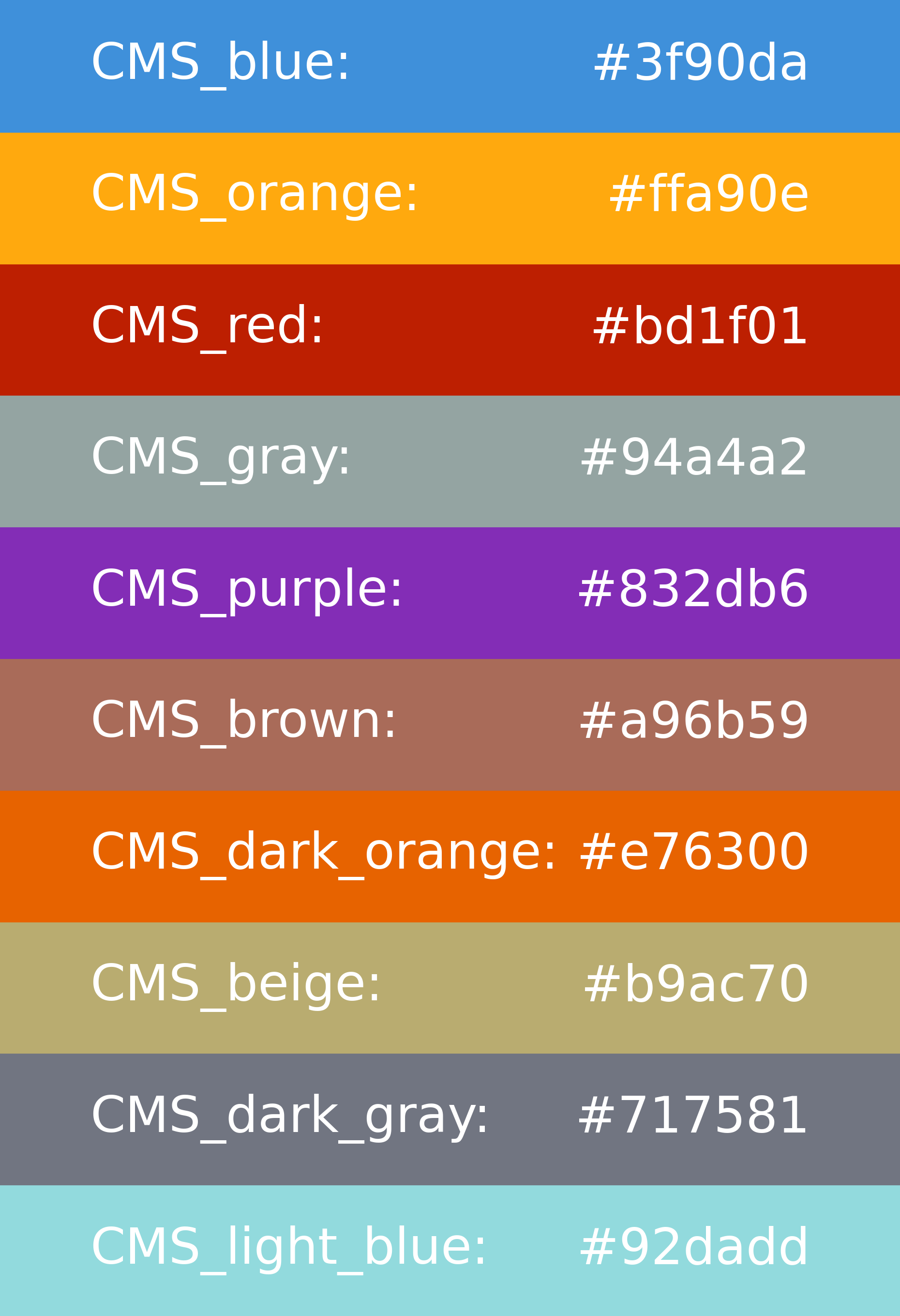
Usage in the .yaml config file:
plotting_style:

    colors_mc:
        TTTo2L2Nu: CMS_red
        TTToSemiLeptonic: CMS_blue
If no alias or default matplotlib color corresponds to the string specified by the user,
an exception is raised.
Additional custom axes#
In order to include an additional custom axis in the plotting, one has to specify the dictionary of categorical axes for data and MC separately.
For example, to include an additional axis for data to keep track of different data-taking eras as an additional category, one can overwrite the custom .yaml file as follows:
plotting_style:

    categorical_axes_data:
        era: eras
where the key (era) in the dictionary corresponds to the name of the axis as saved in the histogram, while the value (eras) corresponds to the name assigned to the corresponding attribute of the Shape object.